When two assets crash together: back-testing risk beyond a single position

Assumed audience: Wealth managers and risk practitioners who want to understand whether their portfolio risk model actually captures what happens when multiple positions fall at the same time. No prior quant knowledge assumed.

Back-testing checks whether a risk model's forecasts are actually correct. Most back-testing does this one asset at a time. But portfolios are made of many assets — and the real question in a crisis isn't whether each position behaved as expected in isolation. It's whether they all moved against you simultaneously.

This article introduces the tool used to capture joint risk, explains why the model most risk systems rely on is structurally blind to this problem, and shows what the data reveals when you test a better model properly — including on market periods it has never seen before.

1. Risk is a forecast and forecasts can be wrong

Every risk model makes a promise. When it tells you the 5% daily VaR on a portfolio is 2%, it's saying: on roughly one trading day in twenty, losses will exceed that number. That's a testable claim. And like any forecast, it should be tested.

Back-testing is how you do it. You replay history, compare predictions to outcomes, and see if the model was right.

In earlier research, Edgelab developed a rigorous way to test whether a single asset's risk forecast is actually correct — not just on average, but consistently, through different market regimes and stress periods. That work showed that the standard approach to back-testing — checking only whether losses exceeded a threshold the right number of times — misses too much. A model can pass that test while being systematically too slow to react when conditions shift. Still showing calm while the storm is already building.

That was the univariate problem: one asset, one forecast, one test.

This research asks the harder question. When two assets are involved, does the model correctly describe how they move together — during the typical days, but also in the tails, when both are having their worst days at the same time?

2. Why one asset at a time isn't enough

Imagine two colleagues who commute separately to work. Anna is late about 20% of the time. Bruno, about 30%. You've tracked both for years. You know each pattern well.

Now someone asks: what's the chance they're both seriously late on the same day?

You can't answer this from what you know about each of them individually. You need something extra: the structure of their relationship. Do they travel through the same part of the city? When a disruption hits, does it reach both routes? When Anna is having her worst morning, does that make Bruno's bad too — or are their commutes essentially unrelated?

Entirely separate from what each does on their own, that extra piece, the dependency, is what determines the answer.

The same logic applies to a portfolio. A risk model can forecast each asset's behavior correctly in isolation and still be wrong about what matters most in a crisis: whether losses arrive together. Positions that each behave within their predicted range can still produce a severe drawdown if they all disappoint simultaneously.

And they tend to. In financial crises, assets that seemed to move somewhat independently in calm markets start moving in lockstep when conditions deteriorate. The diversification you counted on weakens at exactly the moment you need it most.

Testing risk one asset at a time cannot catch this.

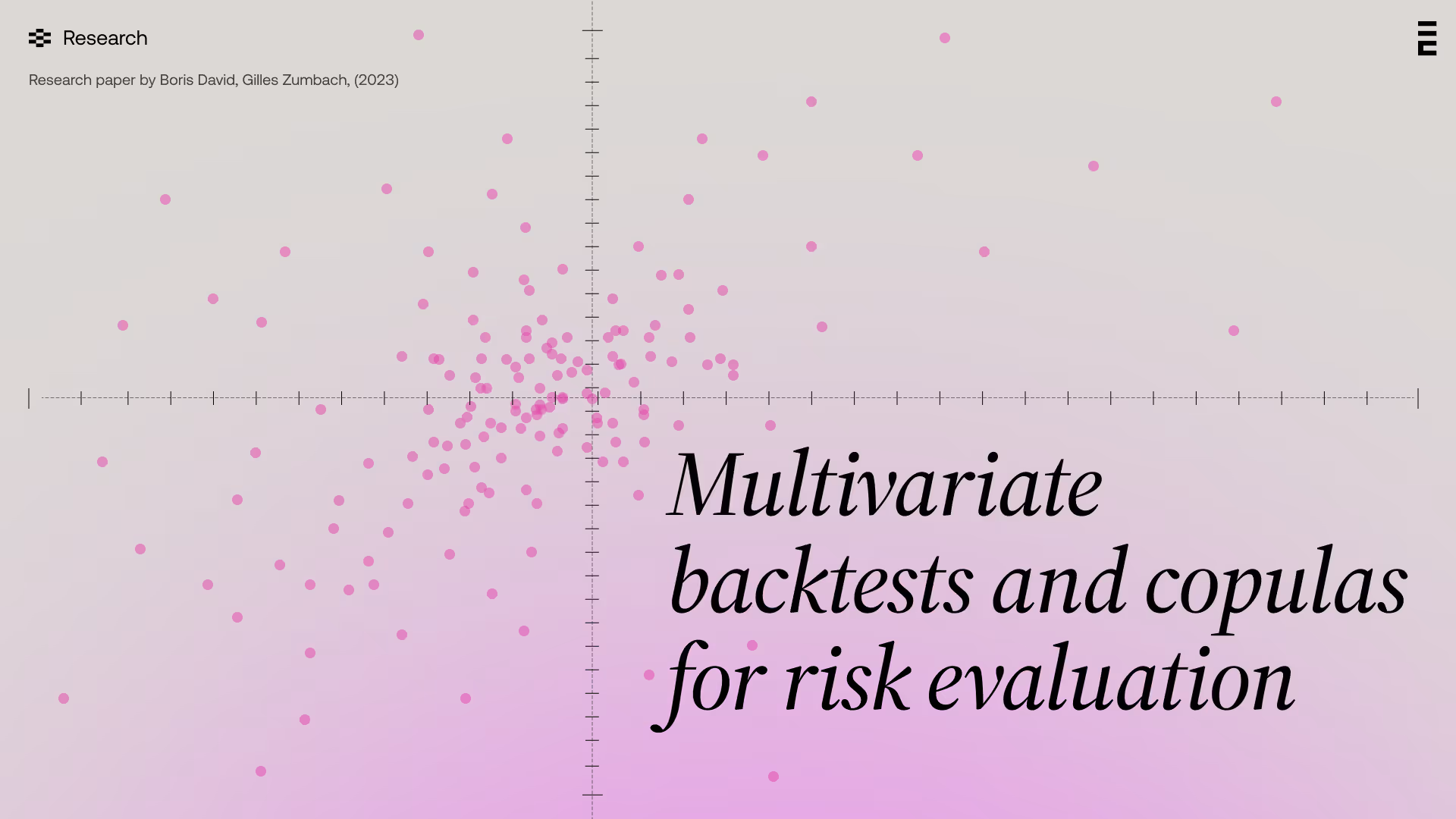
3. The tool that captures joint risk

Any relationship between two random variables can be separated into two pieces.

The first is what each variable does on its own — each asset's individual distribution, its average behavior, its volatility, the shape of its worst days.

The second is how they move together. When one asset is in its worst 10% of days, is the other also in its worst 10%? More often than chance alone would suggest? And does that tendency intensify as things get more extreme?

A copula captures only that second piece. It carries no information about the size of each asset's moves — only the relationship between where each sits in its own distribution on any given day. When one is at its worst, what is the other doing?

This separation makes copulas powerful for risk research. It isolates the question of joint behavior so it can be studied and tested independently. You can ask: does a given structure of dependence between two assets match what history actually shows? And does a forecast built on that structure hold up on data the model has never seen?

Before the test can run, there is one prerequisite worth understanding. Financial markets are not equally volatile at all times. The calm of 2017 and the violence of March 2020 are not drawn from the same statistical world. Running tests on a dataset that mixes these regimes without accounting for the difference is like measuring a typical morning commute by averaging ordinary days with days when the entire transit system has shut down. The average tells you almost nothing useful.

The solution is to divide each day's return by an estimate of how volatile markets were up to the previous day. What remains is the return relative to prevailing conditions — a stable, comparable series. These adjusted observations are called innovations, quantifying the surprises, independently of the market states. Getting this right is not a technical detail. It is the foundation the rest of the analysis depends on. Edgelab uses a long-memory volatility model to do it well: one that recognizes volatility is shaped not just by the past few days move, but by a longer history of market turbulence.

4. The standard model's blind spot

Back to Anna and Bruno. You want to assess the chance they're both badly late on the same day. Here is one first natural assumption: yes, their bad mornings sometimes coincide but truly catastrophic joint days, both of them stuck for hours simultaneously, are occuring just according to chance and not more. When things go really wrong, they usually go wrong for one person at a time.

But they share a city. A transportation failure will likely affect both. Therefore, the previous assumption of independence is too strong: when one is late, the other is more likely to be late. Such events are correlated.

The correlation tells you that they are dependencies: both can be late more often than just by chance. But correlation is only a coarse measure, the full picture for the dependencies is given by the copula. If Anna is very late, how likely is Bruno to be on time, somewhat late, or very late. The correlation can be identical, but the full dependencies different.

A natural measure of dependencies is the Gaussian copula, induced by a multivariate normal distribution. It acknowledges correlations between assets, and assigns low probability to extreme joint events. Simultaneous severe moves in multiple positions are unlikely.

Financial markets don't work this way, the dependencies are larger.

When things go wrong in markets, they tend to go wrong together, more severely and more often than the normal distribution allows for. Assets that moved somewhat independently in calm markets start moving in lockstep during a sell-off. Joint extremes — both assets having their worst days simultaneously — are more common than the Gaussian copula.

An alternative is a Student-t copula, derived from a multivariate Student-t distribution. It acknowledges that large simultaneous moves are a real and recurring feature of financial markets, not an anomaly. And this is not a theoretical preference. It is what the data shows, consistently, across different assets, different correlations and different time periods.

The practical implication is direct. A model that uses Gaussian assumptions about joint behavior underestimates the probability that multiple positions hurt you at the same time. In calm markets, this error is invisible. In a crisis — when you are relying most heavily on your risk numbers — it is exactly the mistake that matters.

5. What the research found

The analysis covered a wide cross-section of asset pairs: equity indexes, currencies, assets with high correlations and low ones, across different market regimes. Two questions drove it.

First: what is the actual structure of joint risk in financial markets — Gaussian or something heavier-tailed?

Second: does a forecast built on that structure hold up on data the model has never seen?

On the first question, the finding is clear and consistent. The Student-t copula describes the joint behavior of financial time series better than the Gaussian, and this holds regardless of the correlation level between the assets. High correlation, low correlation — it doesn't change the result. Financial markets have fatter joint tails than the normal model assumes. This is a stable feature of the data, not a feature of one particular period or one particular market.

On the second question — the harder and more important one — the answer is: yes, it does.

The approach builds forecasts from historical innovations, then adjusted for the current volatility levels. When those forecasts were tested against periods the model had never observed, they held. The joint distributional forecasts were statistically correct. The model does what it claims.

This second result is the one that matters. Fitting a model to historical data and declaring it working is easy. Generating correct predictions about periods the model has never seen — that is the test most risk systems skip. Out-of-sample validation of multivariate forecasts is new. It is also the standard Edgelab's methodology is built to meet.

6. What this means for wealth managers

A correlation figure is a single number. It summarizes how two assets have moved together on average over some historical period. What it doesn't capture is the structure of that relationship, and in particular in the tails — what it looks like when both assets are simultaneously under severe stress. And it doesn't tell you whether that structure was correctly modeled in advance or only described after the fact.

These are not abstract distinctions. They determine whether a risk engine gives you an accurate picture of portfolio behavior in the moments that count — when markets are falling, positions are moving against each other at once and the number on your screen is the thing you're relying on to understand your exposure.

The question worth asking of any risk model — whether built in-house or provided by a partner — is not just what the correlations are. It's what structure the model assumes for joint behavior under stress. And whether that structure has ever been tested on data it has never seen.

Most haven't been tested that way. And Edgelab's methodology passes such very stringent tests. Because a model that underestimates joint tail risk costs clients money at exactly the wrong moment — when a crisis hits and several positions fall together.

Based on the research paper of Boris David and Gilles Zumbach, "Multivariate backtests and copulas for risk evaluation," Edgelab, 2023.

{{cta}}

‍

P.S. The single-asset version of this back-test — and what it reveals about widely used VaR methodologies — is covered in the tile test piece. For the longer horizon question, the article on long-term market simulations looks at whether the models behind decade-scale projections hold up.